Extracting R’s learned LDA model parameters into word cloud visualisations.

R’s topicmodels package contains an LDA function for performing Latent Dirichlet Allocation on a text corpus. LDA separates a text corpus into k topics, assigning each document in the corpus a topic weight. Each topic in turn is represented by a set of term weights. I wanted to display the terms with the highest weight in a word cloud for each topic.

It wasn’t immediately apparent to me how to transform the results of LDA into a format suitable for creating a word cloud, so I’ve set out the missing piece of the puzzle below.

First, let’s run LDA on the example ‘Associated Press’ dataset and create 2 example topics:

library(topicmodels)
library(wordcloud)

data("AssociatedPress")

lda <- LDA(AssociatedPress, k = 2, control = list(seed = 1234))

The k parameter specifies the number of topics we seek to separate the copus into. (For help on choosing an optimal k, take a look at the ldatuning package).

Having created a trained lda object, it’s trivially easy to extract the top terms for each topic using the terms function:

terms(lda, 5)

#      Topic 1   Topic 2
# [1,] "percent" "i"
# [2,] "million" "president"
# [3,] "new"     "government"
# [4,] "year"    "people"
# [5,] "billion" "soviet"

Whilst this is useful for inspecting returned topics, it lacks a key piece of information necessary for creating word clouds: the strength of each word in the topic. It’s not enough to know the rank, we also want to know the weight.

Much of the information about inspecting LDA results understandably focuses on the relationship between topics and documents (LDA after all being primarily a document classification algorithm). The topic-document weights are available in the gamma variable:

head(lda@gamma)

#              [,1]      [,2]
# [1,] 0.2480616686 0.7519383
# [2,] 0.3615485445 0.6384515
# [3,] 0.5265844180 0.4734156
# [4,] 0.3566530023 0.6433470
# [5,] 0.1812766762 0.8187233
# [6,] 0.0005883388 0.9994117

Notice that each row of the gamma matrix sum to 1.0. This contains, the proportion of each document’s weight that should be allocated to each topic.

It wasn’t immediately apparent to me that the beta variable contains the same information for terms. The dimension of the beta matrix is 2 x 10473, or the number of topics x the number of terms. However each column certainly doesn’t sum to 1.0:

lda@beta[,1]

# [1] -27.10812 -10.15299

Nor do the rows:

sum(lda@beta[1,])

# [1] -167587.3

It eventually dawned on me that the values in the beta matrix are actually the log transformation of the actual probabilities. If we transform the values in the other direction, with exp, we discover that in fact the rows do sum to 1.0:

> sum(exp(lda@beta[1,]))

# [1] 1

Thus, we can infer that the beta matrix actually contains the proportion of each topic’s weight that should be allocated to each term. This is exactly the weight we want to plot on our word cloud. We can create a dataframe from the terms and values from the beta matrix corresponding to the topic we’re interested in, and sort by the probability descending:

topic <- 1
df <- data.frame(term = lda@terms, p = exp(lda@beta[topic,]))
head(df[order(-df$p),])

#          term           p
# 6838  percent 0.009806671
# 5957  million 0.006837635
# 6286      new 0.005942985
# 10423    year 0.005750201
# 982   billion 0.004267884
# 5292     last 0.003679708

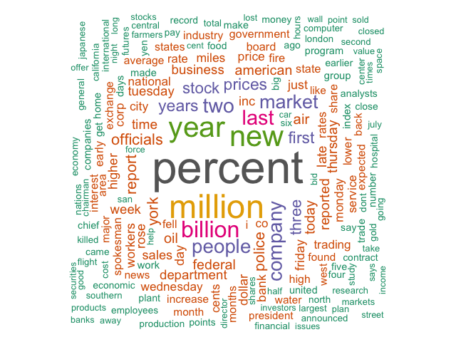
This dataframe is ready for use in R’s wordcloud library like so:

wordcloud(words = df$terms,
          freq = df$p,
          max.words = 200,
          random.order = FALSE,
          rot.per = 0.35,
          colors=brewer.pal(8, "Dark2"))